2014/01/07

Towards the basic R mindset.

Previously

The post “A first step towards R from spreadsheets” provides an introduction to switching from spreadsheets to R.  It also includes a list of additional posts (like this one) on the transition.

Add two columns

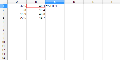
Figure 1 shows some numbers in two columns and the start of adding those two columns to each other in a third column.

Figure 1: Adding two columns in a spreadsheet. 

The next step is to fill the addition formula down the column.

It is not so different to do the same thing in R.  First create two objects that are equivalent to the two columns in the spreadsheet:

A <- c(32.5, -3.8, 15.9, 22.5)
B <- c(48.1, 19.4, 46.8, 14.7)

In those commands you used the c function which combines objects.  You have created two vectors.  The rules for a vector are:

• it can be any length (up to a very large value)
• all the elements are of the same type — all numbers, all character strings or all logicals
• the order matters (just like it matters which row a number is in within a spreadsheet)

To summarize: they’re in little boxes and they all look just the same.

You have two R vectors holding your numbers.  Now just add them together (and assign that value into a third name):

C <- A + B

This addition is precisely what is done in the spreadsheet: the first value in C is the first value in A plus the first value in B, the second value in C is the second value in A plus the second value in B, and so on.

See the values in an object by typing its name:

> C
[1] 80.6 15.6 62.7 37.2

The “> ” is the R prompt, you type only what is after that: ‘C‘ (and the return or enter key).

Also note that R is case-sensitive — C and c are different things:

> c
function (..., recursive = FALSE)  .Primitive("c")

(Don’t try to make sense of what this means other than that c is a function.)

Multiply by a constant

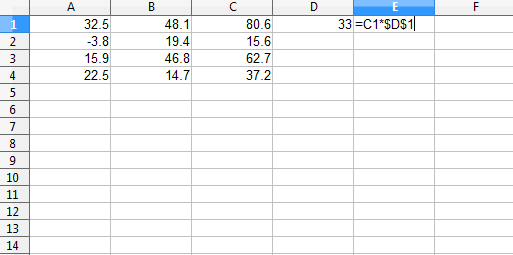
One way of multiplying a column by a constant is to multiply the values in the column by the value in a single cell.  This is illustrated in Figure 2.

Figure 2: Multiply a column times the value in a single cell, shown before filling down column E. 

Another way of doing the same thing is to fill the value in D1 down column D and then multiply the two columns.

Do this operation in R with:

> C * 33
[1] 2659.8  514.8 2069.1 1227.6

In this command you didn’t create a new object to hold the answer.

You can think of R as doing either of the spreadsheet methods, but the fill-down image might be slightly preferable.

Recycling in R

The R recycling rule generalizes the idea of a single value expanding to the length of the vector.  It is possible to do operations with vectors of different lengths where both have more than one element:

> 1:6 + c(100, 200)
[1] 101 202 103 204 105 206

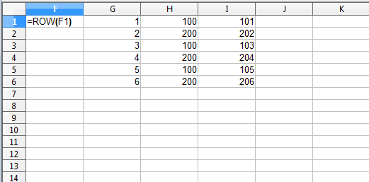
Figure 3 illustrates how R got to its answer.

Figure 3: Equivalent of the example of R’s recycling rule. 

Column F shows how column G was created: use the ROW function and fill it down the column.  That sequence of numbers was created in R with the `:` operator.

Note how the shorter vector is replicated to the length of the longer one.  Each value is used in order, and when it reaches the end it goes back to the beginning again.

You are free to think this is weird.  However, it is often useful.

Functions

Table 1 translates between spreadsheet and R functions. The spreadsheets consulted were Excel, Works and OpenOffice. Note there is some variation between spreadsheets.

Table 1: Equivalent functions between spreadsheets and R.

spreadsheet	R	comment
ABS	abs
ADDRESS		perhaps assign but there is probably a better way
AND	all	more literally would be the & and && R operators
AVERAGE	mean	danger: mean accepts only one data argument
AVG	mean	this danger of mean is discussed in Circle 3 of The R Inferno
AVERAGEIF		subscript before using mean
BESSELI	besselI
BESSELJ	besselJ
BESSELK	besselK
BESSELY	besselY
BETADIST	pbeta
BETAINV	qbeta
BINOMDIST	pbinom or dbinom	pbinom when cumulative, dbinom when not
CEILING	ceiling
CELL		str is sort of the same idea
CHIDIST	pchisq	CHIDIST(x, df) is pchisq(x, df, lower.tail=FALSE)
CHIINV	qchisq	CHIINV(p, df) is qchisq(1-p, df)
CHISQDIST	pchisq or dchisq	pchisq when cumulative, dchisq when not
CHISQINV	qchisq
CHITEST	chisq.test
CHOOSE	switch
CLEAN	gsub
COLS	ncol	(Works)
COLUMNS	ncol	(Excel, OpenOffice)
COLUMN	col	or probably more likely : or seq
COMBIN	choose
CONCATENATE	paste
CONFIDENCE		CONFIDENCE(alpha, std, n) is -qnorm(alpha/2) * std / sqrt(n)
CORREL	cor
COUNT	length
COUNTIF		get length of a subscripted object
COVAR	cov
CRITBINOM	qbinom	CRITBINOM(n, p, a) is qbinom(a, n, p)
DELTA	all.equal or identical	all.equal allows for slight differences, and note that it does not return a logical if there’s a pertinent difference — you can wrap it in isTRUE if you want
DGET		use subscripting in R
ERF		see the example in ?"Normal"
ERFC		see the example in ?"Normal"
EXACT	==	EXACT is specific to text, == is not
EXP	exp
EXPONDIST	pexp or dexp	pexp when cumulative, dexp when not
FACT	factorial
FACTDOUBLE	dfactorial	dfactorial is in the phangorn package
FDIST	pf	FDIST(x, df1, df2) is pf(x, df1, df2, lower.tail=FALSE)
FIND	regexpr
FINV	qf	FINV(p, df1, df2) is qf(1-p, df1, df2)
FISHER	atanh
FISHERINV	tanh
FIXED	format or sprintf or formatC
FLOOR	floor
FORECAST		predict on an lm object
FREQUENCY		you probably want to use cut and/or table
FTEST	var.test
GAMMADIST	pgamma or dgamma	GAMMADIST(x, a, b, TRUE) is pgamma(x, a, scale=b) GAMMADIST(x, a, b, FALSE) is dgamma(x, a, scale=b)
GAMMAINV	qgamma	GAMMAINV(p, a, b) is qgamma(p, a, scale=b)
GAMMALN	lgamma
GAUSS		GAUSS(x) is pnorm(x) - 0.5
GCD	gcd	gcd is in the schoolmath package (and others). For more than two numbers you can do: Reduce(gcd, numVector)
GEOMEAN		exp(mean(log(x)))
GESTEP	>=	GESTEP(x, y) is as.numeric(x >= y) but R often coerces automatically if needed
HARMEAN	harmonic.mean	harmonic.mean is in the psych package
HLOOKUP		use subscripting in R
HYPGEOMDIST	dhyper	HYPGEOMDIST(x, a, b, n) is dhyper(x, b, n-b, a)
IF	if or ifelse	see Circle 3.2 of The R Inferno on if versus ifelse
IFERROR	try or tryCatch
INDEX	[	use subscripting in R
INDIRECT	get	or possibly the eval-parse-text idiom, or (better) make changes that simplify the situation
INT	floor	danger: not the same as as.integer for negative numbers
INTERCEPT		(usually) the first element of coef of an lm object
ISLOGICAL	is.logical
ISNUMBER	is.numeric
ISTEXT	is.character
KURT	kurtosis	kurtosis is in the moments package
LARGE		you can use subscripting after sort
LCM	scm	scm is in the schoolmath package. For more than two numbers you can do: Reduce(scm, numVector)
LEFT	substr
LEN	nchar	(Excel, OpenOffice)
LENGTH	nchar	(Works)
LINEST		use lm
LN	log	danger: the default base in R for log is e
LOG	log	danger: the default base in spreadsheets for log is 10
LOG10	log10
LOGINV	qlnorm
LOGNORMDIST	plnorm
LOWER	tolower
MATCH	match or which	match only does exact matches. Given that MATCH demands a sorted set of values for type 1 or -1, then MATCH(x, vec, 1) is sum(x <= vec) and MATCH(x, vec, -1) is sum(x >= vec) when vec is sorted as MATCH assumes.
MAX	max or pmax	max returns one value, pmax returns a vector
MDETERM	det
MEDIAN	median
MID	substr
MIN	min or pmin	min returns one value, pmin returns a vector
MINVERSE	solve
MMULT	%*%
MOD	%%
MODE		the table function does the hard part. A crude approximation to MODE(x) is as.numeric(names(which.max(table(x))))
MUNIT	diag	diag is much more general
N	as.numeric	the correspondence is for logicals, as.numeric is more general
NEGBINOMDIST	dnbinom
NORMDIST, NORMSDIST	pnorm or dnorm	pnorm when cumulative is true, dnorm when false
NORMINV, NORMSINV	qnorm
NOT	!
NOW	date or Sys.time
OR	any	the or operators in R are | and ||
PEARSON	cor
PERCENTILE	quantile
PERCENTRANK		similar to ecdf but the argument is removed from the distribution in PERCENTRANK
PERMUT		function(n,k) {choose(n,k) * factorial(k)}
PERMUTATIONA		PERMUTATIONA(n, k) is n^k
PHI	dnorm
POISSON	ppois or dpois	ppois if cumulative, dpois if not
POWER	^
PROB		you can use the Ecdf function in the Hmisc package (the probabilities in the spreadsheet are the weights in Ecdf), then you can get the difference of that on the two limits
PRODUCT	prod
PROPER		see example in ?toupper
QUARTILE		use quantile
QUOTIENT	%/%
RAND	runif	see an introduction to random generation in R
RANDBETWEEN		use sample
RANK	rank	RANK has the "min" tie.method and defaults to biggest first. rank only has smallest first. To get biggest first in R you can do: length(x) + 1 - rank(x)
REPLACE	sub or gsub
REPT		use rep and paste or paste0
RIGHT	substring	you’ll also need nchar to count the characters. Alternatively you can use str_sub in the stringr package with negative limits
ROUND	round	note: round rounds exact halves to even (which avoids bias)
ROUNDDOWN	trunc	trunc only goes to integers
ROW	row	or probably more likely : or seq
ROWS	nrow
RSQ		in summary of an lm object
SEARCH	regexpr	also see grep
SIGN	sign
SKEW	skewness	skewness is in the moments package
SLOPE		in coef of an lm object
SMALL		you can use subscripting after sort
SQRT	sqrt
STANDARDIZE	scale
STD	sd	(Works)
STDEV	sd	(Excel, OpenOffice)
STEYX		predict on an lm object
STRING	format or sprintf or formatC or prettyNum	(Works)
SUBSTITUTE	sub or gsub	or possibly paste
SUM	sum	sum is one of the few R functions that allow multiple data arguments
SUMIF		subscript before using sum
SUMPRODUCT	crossprod
TDIST	pt	TDIST(abs(x), df, tails) is pt(-abs(x), df) * tails
TEXT	format or sprintf or formatC or prettyNum
TINV		TINV(x, df) is abs(qt(x/2, df))
TODAY	Sys.Date
TRANSPOSE	t
TREND		fitted of an lm object
TRIM	sub
TRIMMEAN	mean	TRIMMEAN(x, tr) is mean(x, trim=tr/2)
TRUNC	trunc
TTEST	t.test
TYPE		similar concepts in R are typeof, mode, class. Use str to understand the structure of objects
UPPER	toupper
VALUE	as.numeric
VAR	var
VLOOKUP		use subscripting in R
WEEKDAY	weekdays
WEIBULL	pweibull or dweibull	pweibull when cumulative, dweibull when not
ZTEST		use pnorm on the calculated statistic

The trigonometric functions, like cos, acos, acosh are the same, except the R functions are all in lowercase.

Arguments

Spreadsheets show you the arguments of a function.  The args function in R provides similar information.  For example:

> args(sample)
function (x, size, replace = FALSE, prob = NULL) 
NULL

This shows that replace and prob both have default values, and so are not required.  Actually size is not required either — x is the only mandatory argument.

You will learn to not even see the NULL on the final line of the result of args.

Help

You can get help for a function with the question mark operator:

?sample

This will show you the help file for the object — sample in this case.  It is best not to let yourself be overwhelmed by a help file.

R vectorization

Most of the R functions are vectorized.

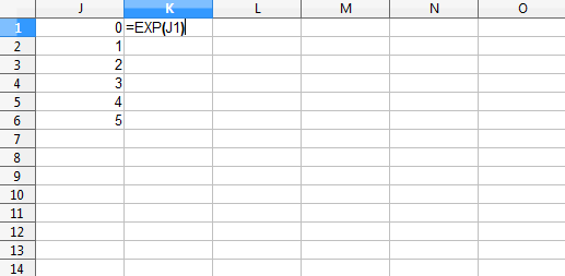
This is like creating a new spreadsheet column where an argument of the function is a value from the same row but a different column.  Think of putting =EXP(A1) in cell B1 and then filling it down.

Figure 4: EXP example of the vectorization idea, shown before column K is filled down. 

Giving a vector to exp returns the exponential of each of the values in the input vector:

> exp(0:5)
[1]   1.000000   2.718282   7.389056  20.085537
[5]  54.598150 148.413159

The result is a vector of length 6 — the same length as the input. The number in square brackets at the start of each line of output is the index number of the first item on the line.

Some R resources

“Impatient R” provides a grounding in how to use R.

“Some hints for the R beginner” suggests additional ways to learn R.

Epilogue

And they’re all made out of ticky tacky
And they all look just the same

from “Little Boxes” by Malvina Reynolds (1900 – 1978)

Tags: Excel, OpenOffice, R versus Excel, R versus spreadsheet, spreadsheets, Works