2014/08/17

Navigation gets you from where you are to where you want to be.

Speaking of navigation, you can jump to selected sections of this post: Navigation; R-bloggers; Task views; Rdocumentation.org; sos package; ??; apropos; ls; methods; getAnywhere; :::; find; args; grep; %in%; str; getwd; file.choose; Spyglass summary; browser; See also.

Overview

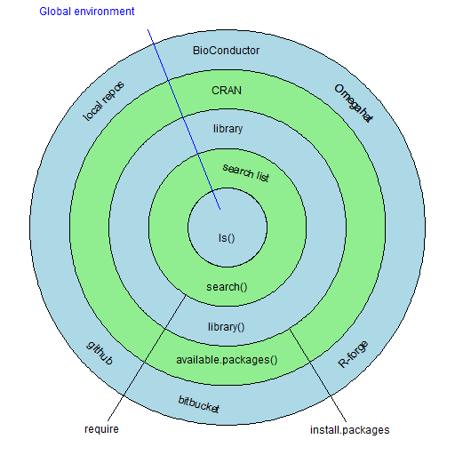
Figure 1: A map of the R world. Each R session has a workspace specific to it. Ironically this is called the global environment.  You can see what objects are in it with the command:

ls()

Or if you prefer explicitness over laziness:

objects()

But your R session will know about other objects as well. Those objects will be in items that are on the search list.  You can see the current state of the search list with:

search()

The items can be packages, or files of R objects (created, for example, via the save function and put on the search list with attach).  It is almost a true statement that R searches for objects in the order of the search list — first in the global environment, then in whatever is second on the search list, and so on.

The packages on the search list will have been selected from the library of packages on your machine.  You see what packages are in your library with:

library()

Add a package to the search list with the require function.  For example to add the BurStMisc package to the search list, you would do:

require(BurStMisc)

The same effect is achieved with:

library(BurStMisc)

There are reasons to dislike each of these — require fails to throw an error if the package is not available, while library conflates both terminology and operations.

The packages in your library have to get there from somewhere.  That somewhere is called a repository.  The main R repository is CRAN.  The function that takes packages from CRAN and puts them into your library is install.packages.  This is used like:

install.packages("BurStMisc")

CRAN is the primary repository, but not the only one.  You can even create your own.

Navigation

Navigation can be broken into a few steps.  Perhaps something like:

• Decide a destination
• Chart a course
• Steer the ship
• Keep track of where you are
• Survive trouble

1) R-bloggers

If you’re not so sure where you want to go, then having a glance through R-bloggers might give you some hints for vacation spots.

Chart a course

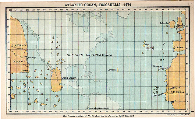
Suppose you are starting on the Iberian peninsula and you want to get to India.  How to do that?

You can go south and then east when you can, like they’ve done for a while now.  Or you can go west instead.

“Atlantic Ocean, Toscanelli, 1474” by Bartholomew, J. G. – A literary and historical atlas of America, by Bartholomew, J. G.. Licensed under Public domain via Wikimedia Commons.

2) Task views

Each Task View outlines the CRAN functionality that is available for that specialty.  The views generally fall into two categories:

• area of study (e.g., Finance or Medical imaging)
• technique (e.g., Machine learning or Optimization)

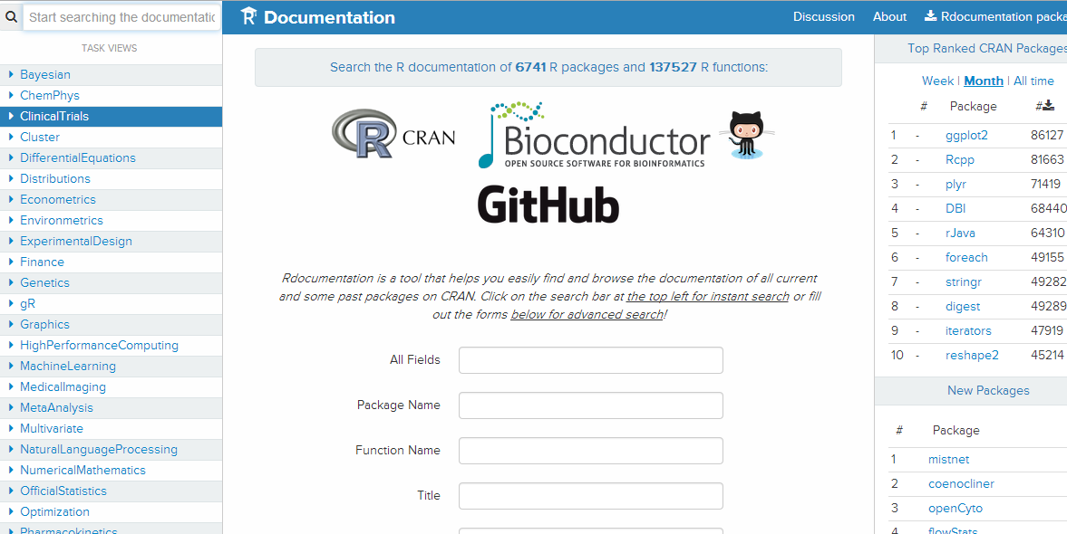
3) Rdocumentation.org

Rdocumentation gathers help files from lots of places and makes them searchable. You can find functionality from the wide world of R here.  Easily.

Note that just because you don’t find what you are looking for, doesn’t mean that it doesn’t exist.  When the name of the strsplit function recently escaped me, I failed to find it here (because I didn’t know the right words to put in the search).

If you come up empty, there is always internet search (but see below).

4) sos package

The sos package performs essentially the same task as Rdocumentation but in a different way.  One difference is that while Rdocumentation starts and ends in a browser, sos starts in R and ends in a browser. (You’ll need to install sos the first time you want to use it, and put it on the search list in each session you’re using it.)

??? is the centerpiece, use it like:

> ???sudoku
found 18 matches; retrieving 1 page

You need to use quotes if there is more than one word:

???"genetic optimization algorithm"

I lied.  You don’t have to end in a browser — you can manipulate the search results in R:

srch <- ???"genetic optimization algorithm"
table(srch$Package)

The ??? operator is an alias for the findFn function.  There’s more information in the R Journal article.

5) ??

Search the help files that are on the search list with ??:

??find

produces a list of help files on the search list that contain the term (“find” in this case) in appropriate sections.

The ?? operator is an alias for the help.search function.

6) apropos

If you know or suspect part of the name of the function you are looking for, use apropos.  For instance if you think the name might contain “split”, do:

apropos("split")

The result is a vector of function names that contain the phrase.

This only looks at objects that are on the search list.

7) ls

A common use is:

ls()

which (when at the R prompt) lists the objects that are in the global environment — the first position on the search list.

Another use is:

ls(2)

This lists the objects that are in the second position of the search list.  The location on the search list can be specified by name rather than number:

ls("package:utils")
ls("file:mystuff.RData")

Another useful argument is pattern, which in my laziness I usually abbreviate to pat.

ls("package:utils", pat="zip")

The pattern argument restricts the output to objects with names that partially match it — a sort of local apropos.

The all.names argument to ls defaults to FALSE.  When it is TRUE, then objects whose names start with a dot are also printed.

As already noted, ls and objects are synonyms.

Steer the ship

“Columbus Fleet 1893 Issue” by US Post Office – US Post Office /Hi-res scan of stamp from private collection by Gwillhickers. Licensed under Public domain via Wikimedia Commons.

8) methods

R’s object-orientation (generic functions and methods) simplifies naive use, but can produce some grief for the semi-naive.

A generic function (examples are print, plot and summary) has methods specific to the class of the object given as the argument to the function (generally the first argument).

The methods function shows you the methods on the search list that are available for a generic function:

> methods(predict)
 [1] predict.ar*                predict.Arima* 
 [3] predict.arima0*            predict.glm 
 [5] predict.HoltWinters*       predict.lm 
 [7] predict.loess*             predict.mlm* 
 [9] predict.nls*               predict.poly* 
[11] predict.ppr*               predict.prcomp* 
[13] predict.princomp*          predict.smooth.spline* 
[15] predict.smooth.spline.fit* predict.StructTS* 

   Non-visible functions are asterisked

You can go the other way as well.  If you have a class and you want to know the generic functions that have methods specific to that class, then use the class argument to methods:

> methods(class="poly")
[1] makepredictcall.poly* predict.poly* 

  Non-visible functions are asterisked

methods is for S3 methods.  Similar functionality is available for S4 methods with showMethods.

methods(print) # 183 methods in my session

But:

> showMethods(print)

Function "print":
 <not an S4 generic function>
> print
function (x, ...) 
UseMethod("print")
<bytecode: 0x000000000a72ef20>
<environment: namespace:base>

The UseMethod means that this is an S3 generic.  However S3 generics can mutate to be both S3 and S4 generic:

> require(Matrix)
Loading required package: Matrix
> print
standardGeneric for "print" defined from package "base"

function (x, ...) 
standardGeneric("print")
<environment: 0x000000001592f3f8>
Methods may be defined for arguments: x
Use showMethods("print") for currently available ones.
> showMethods(print)
Function: print (package base)
x="ANY"
x="diagonalMatrix"
x="sparseMatrix"

9) getAnywhere

You may have noticed that the results of methods includes the phrase “Non-visible functions are asterisked”.  The ocean has a subsurface containing things that are not easily visible.  So does R.

Packages typically make a few functions visible, but functions that are not of general interest are left invisible.  The visible objects are exported.

The predict.poly function is listed as being non-visible.  This is less visible than having a name that begins with a dot — if we do ls of the package where it lives, it won’t appear even with all.names=TRUE:

> ls("package:stats", all.names=TRUE, pat="predict.poly")
character(0)

But at this point we don’t have a way to know what package the function is in.  Enter getAnywhere:

getAnywhere(predict.poly)

shows you the definition of the function and explains where it found it.

If you are interested only in where something lives, then just get the where component:

> getAnywhere(predict.poly)$where
[1] "registered S3 method for predict from namespace stats"
[2] "namespace:stats"

If there were more than one object on the search list with the name, it would show you all of them.  Let’s experiment:

 > predict.poly <- "want cracker"
> getAnywhere(predict.poly)$where
character(0)

What’s going on?  There should be two things by the name, but this is saying we don’t have any now.

> getAnywhere(predict.poly)
no object named ‘want cracker’ was found

Okay, this is making more sense.  Many of the navigational functions, including this one, cater to us slackers by letting us not use quotes where they logically should be.  But in this case we’ve been caught out and need to add the quotes:

> getAnywhere("predict.poly")$where
[1] ".GlobalEnv" 
[2] "registered S3 method for predict from namespace stats"
[3] "namespace:stats"

10) :::

If you want to look at (or use) a non-exported function from a particular package, then you can use the ::: operator.  For example:

stats:::predict.poly

Think of this as giving the family name in front and the given name at the back.

This is the insistent form of the :: operator, which only works for exported objects.  :: is useful for two reasons:

• if there is (possibly) more than one object to be found by that name
• to make code more explicit to humans

Suppose somewhere in a pile of code you run into:

funkyFunction(x, 42)

This will be quite mysterious if you are unaware of funkyFunction.  It would be much less mysterious if the code read:

pinta::funkyFunction(x, 42)

In this form both R and you know that the function lives in the pinta package (actually what you know is that it lives in the pinta namespace, but close enough).

11) find

find gives you the location on the search list of objects with a specific name:

> find("split")
[1] "package:base"

Using the exact name is the default, but the simple.words argument allows a more general search:

> find("split", simple=FALSE)
[1] "package:graphics" "package:base"

We can investigate further to see the partial matches:

> ls("package:graphics", pat="split")
[1] "split.screen"

12) args

To see the arguments (and their default values) of a function, use args:

> args(find)
function (what, mode = "any", numeric = FALSE, simple.words = TRUE) 
NULL

The args function can be thought of as an alternative to the ? operator.  The command:

?find

produces the help file for the find function.

One of my favorite uses of ? (when sos is on the search list) is:

?"???"

And if sos isn’t on the search list, it’s even better with its amusing (and wrong) suggestion of what to try.

The ? operator is an alias for the help function.

Why would you use args instead of `?`?  At least two reasons:

• you only want a reminder of argument names or defaults
• there isn’t a help file

The latter is often the case (probably too often) for functions written locally.

If a function has a zillion arguments, then it can be hard to find the argument that you care about in the results of args.  There’s a solution for that too.

Suppose you want to find the default value for the fill argument to read.table and you are having a hard time finding it in the results of args.  Then do:

> formals(read.table)[["fill"]]
!blank.lines.skip
> formals(read.table)[["blank.lines.skip"]]
[1] TRUE

Note that by default you need to give the full name of the argument:

> formals(read.table)[["blank"]]
NULL
> formals(read.table)[["blank", exact=FALSE]]
[1] TRUE

The last command uses the exact argument to subscripting to say that it is allowable to give an abbreviation.

If you are having a hard time with the argument names, you can do something like:

> sort(names(formals(read.table)))
 [1] "allowEscapes"     "as.is"            "blank.lines.skip"
 [4] "check.names"      "col.names"        "colClasses" 
 [7] "comment.char"     "dec"              "encoding" 
[10] "file"             "fileEncoding"     "fill" 
[13] "flush"            "header"           "na.strings" 
[16] "nrows"            "numerals"         "quote" 
[19] "row.names"        "sep"              "skip" 
[22] "skipNul"          "stringsAsFactors" "strip.white" 
[25] "text"

13) grep

If you are looking for some bit of text within the strings of a character vector, then use grep:

> grep("na", names(formals(read.table)), value=TRUE)
[1] "row.names" "col.names" "na.strings" 
[4] "check.names"

By default the result of grep is the indices of the strings that match rather than the strings themselves — hence value=TRUE in the call.

14) %in%

If instead of partial matches, you want exact matches, then %in% returns a logical vector stating if the corresponding element of the first vector is an element of the second.

> c("a", "AA", "bb", "aaa", "aa") %in% c("aa", "bb")
[1] FALSE FALSE TRUE FALSE TRUE

%in% uses match which can perform all sorts of magic.

Keep track of where you are

It is popular understanding that Columbus was the first to go west to get to India because of the then belief that the earth is flat.  It was Washington Irving in 1828 who spread that idea.  Actually Columbus was first because others thought — correctly — that India was too far away going west.

15) str

One reason that R is good at what it does is its richness of data structures.  str produces a map of an R object.

Here are a few examples to clue you in:

> str(1:100)
 int [1:100] 1 2 3 4 5 6 7 8 9 10 ...

says it is a length 100 vector ([1:100]) of integers (int), and lists the first few values.

> str(matrix(c(1,2:6),2))
 num [1:2, 1:3] 1 2 3 4 5 6

says that it is a matrix with 2 rows and 3 columns ([1:2, 1:3]) of numeric values (num), and lists all the values.

> str(array(as.character(1:6), c(2,3), list(c("r1", "r2"), NULL)))
 chr [1:2, 1:3] "1" "2" "3" "4" "5" "6"
 - attr(*, "dimnames")=List of 2
  ..$ : chr [1:2] "r1" "r2"
  ..$ : NULL

The first line says it is a matrix with 2 rows and 3 columns ([1:2, 1:3]) of character values (chr), and lists the values.  The second line says that the object has an attribute called “dimnames” that is a list of length 2.  The third and fourth lines give the two components of dimnames.  The first component is a character vector of length 2, and the second component is NULL.

> str(data.frame(matrix(c(1,2:6),2)))
'data.frame': 2 obs. of 3 variables:
 $ X1: num 1 2
 $ X2: num 3 4
 $ X3: num 5 6

The first line says that it is a data frame with 2 rows and 3 columns.  Each of the remaining lines gives the name of the column and its contents.

16) str

str is useful enough to count twice.

17) getwd

R has a sense of where it is.  That location is called the working directory.  Path names to files are understood to be relative to the working directory.  You can see the working directory with:

> getwd()
[1] "C:/Users/pat/burns-stat3/webpages/blog/simple"

Change the working directory with setwd.

18) file.choose

It is not at all unusual for me to need to specify a file name but R and I disagree — that is, what I specify doesn’t exist.  Rather than fixing my mess, it is often easier to use file.choose to print out the path and then paste the result to where I want.

Do:

file.choose()

which gives you a popup window to select the file.  The result is a character string.

Spyglass summary

Table 1 attempts to summarize how to find things in R, though some of the pegs don’t quite fit their holes.  For example, the line for global environment could apply to any item on the search list.

Table 1.

Universe	Partial	Exact	Information
internet	search engine	search engine	search engine
R repositories	Rdocumentation.org	Rdocumentation.org	Rdocumentation.org
CRAN	???	???	???
search list	apropos (name)	find (location)	??
global environment	pattern in ls (name)		? args str
object	grep (indices or strings)	%in% (logical)	str

Survive trouble

The Santa Maria ran aground and met its end on Christmas Day 1492.  Bad things happen — even to brave explorers.

19) browser

I was really proud of myself last week when I wrote a function that worked the first time.  Almost always something is not right with my newly minted functions.  A useful technique to find trouble — or to check if there is trouble — is to put:

browser()

at strategic spots in the function.

When the function is run, then the browser call puts you into the frame of the function.  Do:

ls()

to see the names of the objects in the frame.

You can execute commands as if you are in the function — including making assignments.  To continue the computation, type:

c

as in “continue”.  To quit the computation and get back to the R prompt, type:

Q

as in “Quit”.

An alternative to browser is recover, used like:

recover()

The difference is that recover allows you to look not only inside the frame of the function in which it was called, but in the frames of the chain of functions that led to the call.  If you put the call to recover in function foo, and foo was called by funB which was called by funA, then you can look in the frames of foo, funB and funA.

In this case you are given a numbered menu and you select the number you want, or 0 to exit.  Once you’ve selected a number, it is just like being in browser.  If you say “c” to end the browser session, then you get back to the menu.

20) The R Inferno

The R Inferno charts quite a few rocks that you might run aground upon.

21) Hacking attitude

An important tool to get around in R is to have  a hacking attitude — to try things with the idea that they probably won’t work.  With enough hacking you might even do a columbus — have a great result for the wrong reason.

If you’re looking for spice and you find gold, don’t ignore it.

See also

An introduction to R is “Impatient R”.

Pertinent chapters of Tao Te Programming include: profit from mistakes (Ch. 11), hacking (Ch. 18).

The Wikipedia article on Columbus fails to paint him as the heroic figure I was taught in elementary school.  I wonder which is more accurate.

Updates

22) sessionInfo

The sessionInfo function tells you a variety of information about the current state of your session.  Not least is the versions of the packages that you are using.

> sessionInfo()
R Under development (unstable) (2014-07-29 r66272)
Platform: x86_64-w64-mingw32/x64 (64-bit)

locale:
[1] LC_COLLATE=English_United Kingdom.1252 LC_CTYPE=English_United Kingdom.1252 
[3] LC_MONETARY=English_United Kingdom.1252 LC_NUMERIC=C 
[5] LC_TIME=English_United Kingdom.1252 

attached base packages:
[1] stats graphics grDevices utils datasets methods base 

other attached packages:
[1] Matrix_1.1-4

loaded via a namespace (and not attached):
[1] grid_3.2.0 lattice_0.20-29 tools_3.2.0

Epilogue

And they’ll never know the gold
Or the copper in your hair
How could they weigh the worth
Of you so rare

– from “World before Columbus” by Suzanne Vega

Appendix R

The code to draw Figure 1 is:

P.Rmap <- function (filename = "Rmap.png") 
{
 if(length(filename)) {
  png(file=filename, width=512, height=512)
  par(mar=rep(1, 4) + .1, xpd=TRUE)
 }
 plot.new()
 plot.window(c(-1, 1), c(-1, 1), asp=1)
 theta <- seq(0, 2 * pi, length=400)
 xy <- cbind(cos(theta), sin(theta))
 polygon(xy, col="lightblue")
 polygon(xy * .8, col="lightgreen")
 polygon(xy * .6, col="lightblue")
 polygon(xy * .4, col="lightgreen")
 polygon(xy * .2, col="lightblue")
 text(0, .7, "CRAN")
 text(0, .9, "BioConductor")
 text(xy[50,1] * .9, xy[50,2] * .9, "Omegahat", srt=-45)
 text(xy[350,1] * .9, xy[350,2] * .9, "R-forge", srt=45)
 text(xy[150,1] * .9, xy[150,2] * .9, "local repos", srt=45)
 text(xy[250,1] * .9, xy[250,2] * .9, "github", srt=-45)
 text(xy[290,1] * .9, xy[290,2] * .9, "bitbucket", srt=-15)
 text(xy[50,1] * .9, xy[50,2] * .9, "Omegahat", srt=-45)
 text(xy[80,1] * .3, xy[80,2] * .3, "search list", srt=-15)
 text(xy[100,1] * .5, xy[100,2] * .5, "library")
 text(xy[300,1] * .3, xy[300,2] * .3, "search()")
 text(xy[300,1] * .5, xy[300,2] * .5, "library()")
 text(xy[300,1] * .67, xy[300,2] * .67, "available.packages()")
 text(0, -0.05, "ls()")
 text(-.95, 1.1, "Global environment", 
  col="blue", adj=0)
 segments(xy[125,1] * 1.08, xy[125,2] * 1.08, 
  xy[125,1]*.1, xy[125,2] * .1, col="blue")
 segments(xy[335,1] * 1.15, xy[335,2] * 1.15, 
  xy[335,1]*.6, xy[335,2] * .6, col="black")
 text(xy[335,1] * 1.2, xy[335,2] * 1.2, "install.packages")
 segments(xy[265,1] * 1.15, xy[265,2] * 1.15, 
  xy[265,1]*.4, xy[265,2] * .4, col="black")
 text(xy[265,1] * 1.2, xy[265,2] * 1.2, "require")
 if(length(filename)) {
  dev.off()
 }
}